Topic — Physics on a grid of points: boundary conditions
Needs: Lesson 11 — A grid of blocks: halo exchange and what it costs.
A simulation on a grid has to say what lies beyond its edge. On the wafer that answer comes from the moat: the ring of PEs around the grid. This topic runs three programs, each with one grid point per PE:
| Directory | Physics | Boundary |
|---|---|---|
wave/ | the wave equation | fixed at 0 (Dirichlet), or no flux across the edge (Neumann) |
periodic/ | the same wave equation | periodic: the grid is a torus |
gray-scott/ | Gray-Scott reaction-diffusion, two fields | no flux |
One point per PE keeps the physics easy to follow, but it leaves most of each PE idle; lesson 11 shows why a real solver gives each PE a block. The boundary methods are the same for blocks: the moat answers a whole edge instead of one value.
What you will be able to do
- Set a fixed or a no-flux boundary by what the moat PEs send back.
- Wrap a grid into a torus with moat routers that turn routes around, with no code on the moat.
- Explain why the colorpair layout of lessons 8 and 11 cannot wrap, and lay out colors that alternate from PE to PE instead.
- Exchange two fields per step without mixing them up on shared sockets.
The wave equation (wave/)
The program solves ∂²u/∂t² = c²∇²u by the leapfrog scheme
u_new = 2*u - u_old + alpha * (u_L + u_R + u_D + u_U - 4*u)
where u_L, u_R, u_D and u_U are the four neighbours' values and alpha = c²Δt²/Δx² = 0.25. The
scheme is stable for alpha ≤ 0.5. The field starts as a Gaussian pulse in the middle of the grid,
with u_old = 0, which gives every point an initial velocity equal to its starting value.
The layout
It is the colorpair layout of lesson 11 with one value per PE: a (W+2) × (H+2) rectangle, the
beach, carries the routing of four colorpairs. The interior W × H runs wave.w, and the ring around it, the
shore, runs moat.w:
  +--------------------------------+
  |  shore: moat.w                 |
  |   +----------------------+     |
  |   |  interior W x H      |     |
  |   |  wave.w              |     |
  |   +----------------------+     |
  |                                |
  +--------------------------------+
Each socket sends one way and receives from the opposite side: a sends right and receives from
the left, b sends left, c up and d down. Each step exchanges val with all four neighbours
in one parallel block:
        parallel {
            a[]          <- val;
            b[]          <- val;
            c[]          <- val;
            d[]          <- val;
            u_from_left  <- a[];
            u_from_right <- b[];
            u_from_below <- c[];
            u_from_above <- d[];
        }
and then updates:
        laplacian <- (u_from_left + u_from_right + u_from_below + u_from_above)
                    - 4.0:sp * val;

        sp u_new;
        u_new <- 2.0:sp * val - val_old + alpha * laplacian;
The PE also stores val after every step in history, which display.py reads back.
A boundary condition is an answer
A grid PE at the edge sends its value into the moat, like any other send, and waits for an answer
on the paired socket. What the moat sends back is the value the edge PE uses for its missing
neighbour. moat.w runs four dispatch blocks, one per socket
(lesson 7):
    forever dispatch(b) {
        wavelet(sp v) {
            if (ECHO == 1) a[] <- v;
            else a[] <- 0:sp;
        }
    }
A value that arrives from the right on b came from a grid PE to the moat's right. The answer
leaves on a, which carries it right, back to that PE.
ECHO=0: answer 0. The missing neighbour is 0, so u = 0 on the boundary. This is a Dirichlet condition: the value at the boundary is fixed.ECHO=1: send the value back. The missing neighbour equals the edge point itself, so the difference across the edge is 0 and nothing flows through it. This is a Neumann condition with zero flux, and the sum of u over the grid changes as it would with no boundary at all.
The two rows of wave/test.rc differ only in ECHO:
| Row | Grid | Steps | Moat answers |
|---|---|---|---|
tutorial | 12 × 12 | 50 | 0 |
echo | 12 × 12 | 50 | the value |
ref.py repeats the kernel's SP arithmetic in the same order, with the grid padded by zeros or by
copies of the edge, and the test compares the final u byte for byte. Every product in the update
(×4, ×2, ×0.25) is exact, so the fused multiply-adds that Carbide uses give the same bits as
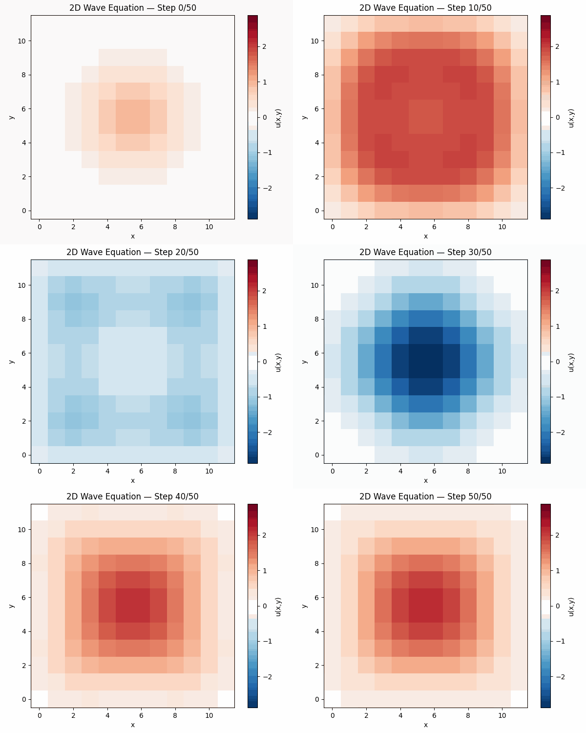
ref.py's separate operations. The mean of u over the grid starts at 0.1737. After 50 steps it is
0.8042 with ECHO=0 and 8.8579 with ECHO=1, which is 51 times the start: with no flux,
leapfrog adds the initial velocity's mean at every step.
The animation shows the tutorial row:
Periodic boundaries (periodic/)
On a torus the right neighbour of the last column is the first column, and the neighbour above the top row is the bottom row. The heat-equation application in the Aviary wraps its grid with moats that turn routes around, and this program does the same for the wave equation.
Why the colorpair layout cannot wrap
In the beach, each direction uses one colorpair. A PE writes socket a; its router moves the
wavelet onto ap, the color on the link (ap [CXR|R]); the neighbour's router moves it back onto
a for its core (a [L|LXC]). So both colors of the pair are in use at every router.
To wrap, the moat at the right end would have to turn ap around onto a color that travels back
left across the whole row. Paint swaps a wavelet only onto the color's partner, and the partner
of ap is a, which every grid router already uses. Turning around needs a color whose partner is free.
Colors that alternate
Without swaps, a color that carries data right has one route per PE: either the PE sends on it
([C>R]) or it receives on it ([L>C]). Two colors that alternate along the row give every PE
both. Grid column gx sends right on r0 if gx is even and on r1 if it is odd, and receives from
the left on the other one. Leftward, upward and downward data alternate in the same way, on l0
and l1, u0 and u1, d0 and d1. For a row of four PEs:
        left moat     gx=0         gx=1         gx=2         gx=3     right moat
            |  --r1-->  |  --r0-->  |  --r1-->  |  --r0-->  |  --r1-->  |
            |  <--l0--  |  <--l1--  |  <--l0--  |  <--l1--  |  <--l0--  |
            |  <================== r1x (back to the left) ========  |
            |  ================== l0x (back to the right) =======>  |
W is even, so the last column sends right on r1 and the first column receives from the left on
r1. That is the one rightward color that leaves the grid. The right moat turns it around onto its
partner r1x, which crosses the row to the left moat, and the left moat turns it back onto r1,
into column 0. Leftward data leaves column 0 on l0 and wraps the other way on l0x. The
vertical directions wrap on u1x and d0x. Paint stops with W must be even or
H must be even otherwise.
The kernel: one socket per direction and way
The alternating colors mean a PE sends right on one color and receives from the left on another,
so periodic/wave.w has eight sockets instead of four:
socket to_r;
socket from_l;
socket to_l;
socket from_r;
socket to_u;
socket from_d;
socket to_d;
socket from_u;
The rest of the kernel is wave/wave.w without history; the exchange sends on the four to_
sockets and receives on the four from_ sockets.
The layout
A grid PE has one of four kinds, by the parity of its column and row. A Paint function makes one PE of a kind, with its eight colors as arguments:
define cell(x y nm tr fl tl fr tu fd td fu) {
    let t = rect(x y 1 1)
    t : code('wave [to_r:tr from_l:fl to_l:tl from_r:fr
                    to_u:tu from_d:fd to_d:td from_u:fu N:N])
    t : paint(tr [C>R])
    t : paint(fl [L>C])
    t : paint(tl [C>L])
    t : paint(fr [R>C])
    t : paint(tu [C>U])
    t : paint(fd [D>C])
    t : paint(td [C>D])
    t : paint(fu [U>C])
    t : name(nm)
    t
}
A 2×2 block holds one PE of each kind, and hstackrep and vstackrep repeat it over the grid:
let block = union(cell(0 0 'c00 r0 r1 l0 l1 u0 u1 d0 d1)
                  cell(1 0 'c10 r1 r0 l1 l0 u0 u1 d0 d1)
                  cell(0 1 'c01 r0 r1 l0 l1 u1 u0 d1 d0)
                  cell(1 1 'c11 r1 r0 l1 l0 u1 u0 d1 d0))
block : hstackrep(W/2 0 'x)
block : vstackrep(H/2 0 'y)
block : place(1 1)
The 0 is the spacing between copies, and 'x and 'y name the replicated dimensions, as in
lesson 11. With a name, a dimension stays in bench.map even when W or H is 2 and the block is
repeated once; the narrow row (W = 2) needs that, because the Makefile always reads the field
with order="y x n _word".
The return colors cross the grid on plain routes:
let grid = rect(1 1 W H)
grid : paint(r1x [R>L])
grid : paint(l0x [L>R])
grid : paint(u1x [U>D])
grid : paint(d0x [D>U])
Turning a route around
The right moat is a column of PEs with routes and no code:
let right = rect(W+1 1 1 H)
right : paint(r1  [LXL])
right : paint(r1x [LXL])
right : paint(l0  [LXL])
right : paint(l0x [LXL])
r1x [LXL] makes r1x take its partner r1 arriving from the left and send it back left.
r1 [LXL] makes r1 read r1x from the left, so that r1 does not also claim the arriving
r1 wavelets. Both rules are needed: without r1 [LXL] the run stops after a few steps
(checked). The second pair works the same way in the other direction: l0x arrives from the left
after crossing the row and leaves as l0, into the last column. The other three moats are the
mirror images, and colorpair makes each pair partners:
let all = union(block grid right left top bottom)
all : colorpair(r1 r1x)
all : colorpair(l0 l0x)
all : colorpair(u1 u1x)
all : colorpair(d0 d0x)
The architecture notes draw this turnaround in Color Swapping, step 4.
Data in and out
Each kind of PE is a separate compile of wave.w, with its own name: a name on the whole grid
would expose only one kind's symbols (lesson 9). So the field is loaded and read in four parts.
init.py writes the whole field and, for each kind cIJ, the points with gx % 2 = I and
gy % 2 = J; the Makefile loops over the four:
KINDS = c00 c10 c01 c11
bench.img: bench.obj init-u.bin bench.map
	cp $< $@
	for k in $(KINDS); do \
	  miset image=$@ out=$@ map=bench.map symbol=$$k.u order="y x n _word" data=init-u-$$k.bin || exit 1; \
	  miset image=$@ out=$@ map=bench.map symbol=$$k.u_old order="y x n _word" data=init-u_old-$$k.bin || exit 1; \
	done
ref.py computes the same steps with np.roll, so the neighbours wrap, and the test compares
each part byte for byte. show.py prints the start and the end. The pulse starts on grid point
(0, 0), so it straddles all four corners:
--- initial u: mean 0.1734 ---
##=:.   .:=#
+=-.     .-=
::.       .:
..         .


..         .
::.       .:
+=-.     .-=
##=:.   .:=#
@#+:.   .:+#
Each frame is scaled to its own range and printed top row first. After 50 steps the mean is 8.8436, again 51 times the start: on a torus nothing leaves.
The rows of periodic/test.rc:
| Row | Grid | Steps |
|---|---|---|
tutorial | 12 × 12 | 50 |
rect | 8 × 6 | 30 |
narrow | 2 × 4 | 20 |
Two fields: Gray-Scott (gray-scott/)
The Gray-Scott model has two chemicals, a substrate U and an activator V, which diffuse and react:
The program takes Euler steps with Δt = Δx = 1, on wave/'s layout, with the echo moat: the
chemicals cannot leave the grid. Its moat.w is wave/moat.w with ECHO=1 built in.
Two exchanges per step
Each step needs both fields from all four neighbours. The kernel exchanges U in one parallel
block and then V in a second:
        // Exchange U, then V, so that each socket carries U before V.
        parallel {
            a[] <- μ;
            b[] <- μ;
            c[] <- μ;
            d[] <- μ;
            μ_L <- a[];
            μ_R <- b[];
            μ_D <- c[];
            μ_U <- d[];
        }

        parallel {
            a[] <- ν;
            b[] <- ν;
            c[] <- ν;
            d[] <- ν;
            ν_L <- a[];
            ν_R <- b[];
            ν_D <- c[];
            ν_U <- d[];
        }
Both fields travel on the same four sockets, and a receiver can tell them apart only by their
order. The arms of one parallel block have no order among them, so two sends on a in one block
could leave in either order. The first block ends before the second starts, so every socket
carries U and then V, and the moat echoes them in that order.
Greek identifiers
The kernel names its variables as the equations do: μ and ν for the local U and V, δ_U,
δ_V, φ and κ for the coefficients, ∇²μ for a Laplacian. Tungsten accepts Greek letters and
superscripts in identifiers
(Greek letters in identifiers).
The check
Carbide fuses a + x * y and a - x * y into one multiply-add with a single rounding
(floating-point evaluation).
ref.py does the same with its fma32 function, which rounds each fused result once to SP, so
its fields match the simulator's bit for bit. The only operation it leaves unfused is the
Laplacian's - 4 * f, which is exact.
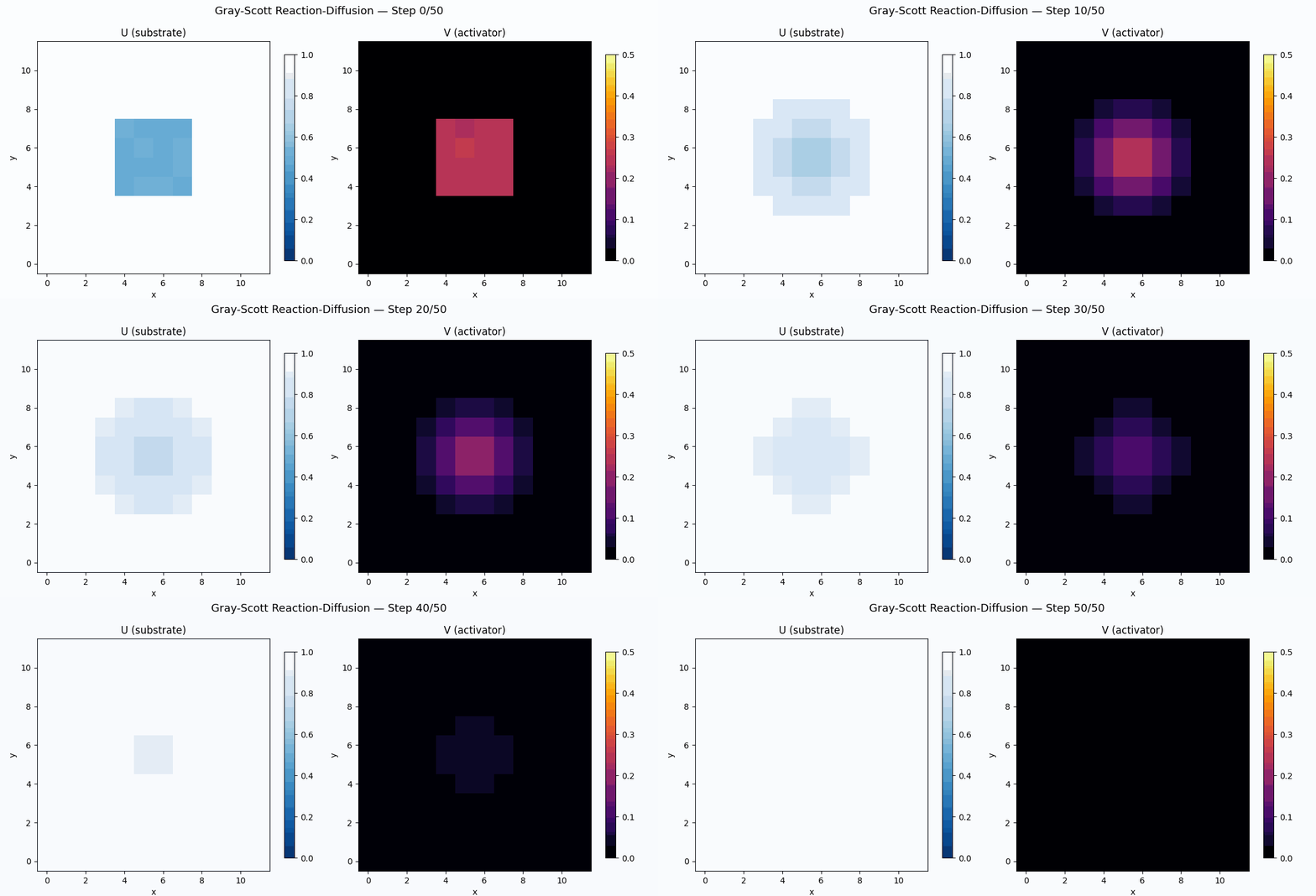
The tutorial row runs 50 steps on a 12 × 12 grid from a seed square in the middle. On a grid this
small, V spreads out and dies away: its largest value falls from 0.26 at the start to 0.011 after
50 steps.
What the hardware does
The moat costs a task per value. Each value that reaches a wave/ moat PE starts a short task
that sends one wavelet back. The edge PE's receive waits for that answer like any other neighbour's
value, so the boundary needs no special case in wave.w.
A wrap uses no core. In periodic/, the moat routers change a wavelet's color and send it back,
and the return color crosses the grid without entering a core. A horizontal wrap takes W + 3 hops instead
of one: into the moat, back across the row to the other moat, and into the first column. A
vertical wrap takes H + 3. It shares
the links with the grid's own traffic. The last memory write of each
run:
| Program | Row | Grid, steps | Last write (cycle) |
|---|---|---|---|
wave | tutorial | 12 × 12, 50 | 7,144 |
wave | echo | 12 × 12, 50 | 7,144 |
periodic | tutorial | 12 × 12, 50 | 7,461 |
periodic | rect | 8 × 6, 30 | 4,326 |
periodic | narrow | 2 × 4, 20 | 2,875 |
gray-scott | tutorial | 12 × 12, 50 | 14,146 |
A step of the wave equation takes about 140 cycles, and Gray-Scott's two exchanges and longer update about twice that.
Budget. Per grid PE, from the compiled kernels:
wave, gray-scott | periodic | |
|---|---|---|
| Colors | 8 | 12 |
| Input queues | 4 receive sockets, each doubled: all 8 queues' storage | the same |
| Output queues | 4 | 4 |
| Microthreads | 8, one per transfer of the exchange | 8 |
Run it
In your copy of the tutorial (see Lesson 1):
cd tutorial/ext-algorithms/grid-physics
make TEST=tutorial               # the tutorial row of each program
cd wave
make TEST='*'                    # both rows of the wave program
make test-tutorial/test          # runs the tutorial row again and prints its snapshots
Each passing row prints one line, such as
wave : 0:06.69 PASS tutorial [ N=50 W=12 H=12 ECHO=0 ARCH=sdr ]. A failing row prints FAIL,
and its make-log ends with cmp naming the first byte where the simulator's field differs from
ref.py's, such as sim-u.bin ref-u.bin differ: byte 1, line 1. A program that stops early fails
the same way: the kernel writes u only at the end, so u still holds its starting values. Run make clean after you edit a source file: make
reuses an existing test-*/ directory. make test-tutorial/animate writes the animation's frames
when matplotlib is installed.
Pitfalls
- One moat swap rule is not enough. A moat that turns a route around needs the rule on both colors of the pair.
- Name the replicated dimensions. With
hstackrep(W/2)and no'x, thenarrowrow fails withorder: 'x' is not a name or number(checked), because a dimension repeated once is left out ofbench.map(lesson 11). - An odd W or H cannot wrap. The color that leaves the last column would not be the one the
first column receives.
bench.paintasserts that both are even. - Two fields on one socket need an order. Keep each field's sends in its own
parallelblock, or give each field its own sockets and colors. - A dispatch moat must answer every value. In
wave/, an edge PE's receive from the moat is an ordinary receive. A moat handler that sends nothing leaves the edge PE waiting forever. - Memory grows with the history.
wave.wkeeps N+1 SP values andgrayscott.w2·(N+1) in every PE, in the 48 KB shared with code. A long run must record fewer steps.
Exercises
- In
wave/moat.w, make the moat answer-vinstead of 0 whenECHO=0, and changeref.pyto pad with the negated edge. This puts the zero halfway between the edge point and the moat. Runmake cleanand thetutorialrow, and compare the snapshots with the original. - In
periodic/, make the grid periodic up and down but fixed at the sides. Replace the right and left moats' turnaround rules with a dispatch moat that answers 0: write a moat kernel with one receive socket and one send socket, give each side moat itscode()and routes, and changeref.pyto pad the left and right with 0 and roll only along y. Which colors does each new moat receive and send on?
Next
Topic — Command streams: Tetris on a column drives a column of PEs with a stream of commands.