Particle-in-Cell on a Wafer: an Electromagnetic Plasma Code Written by an AI Agent

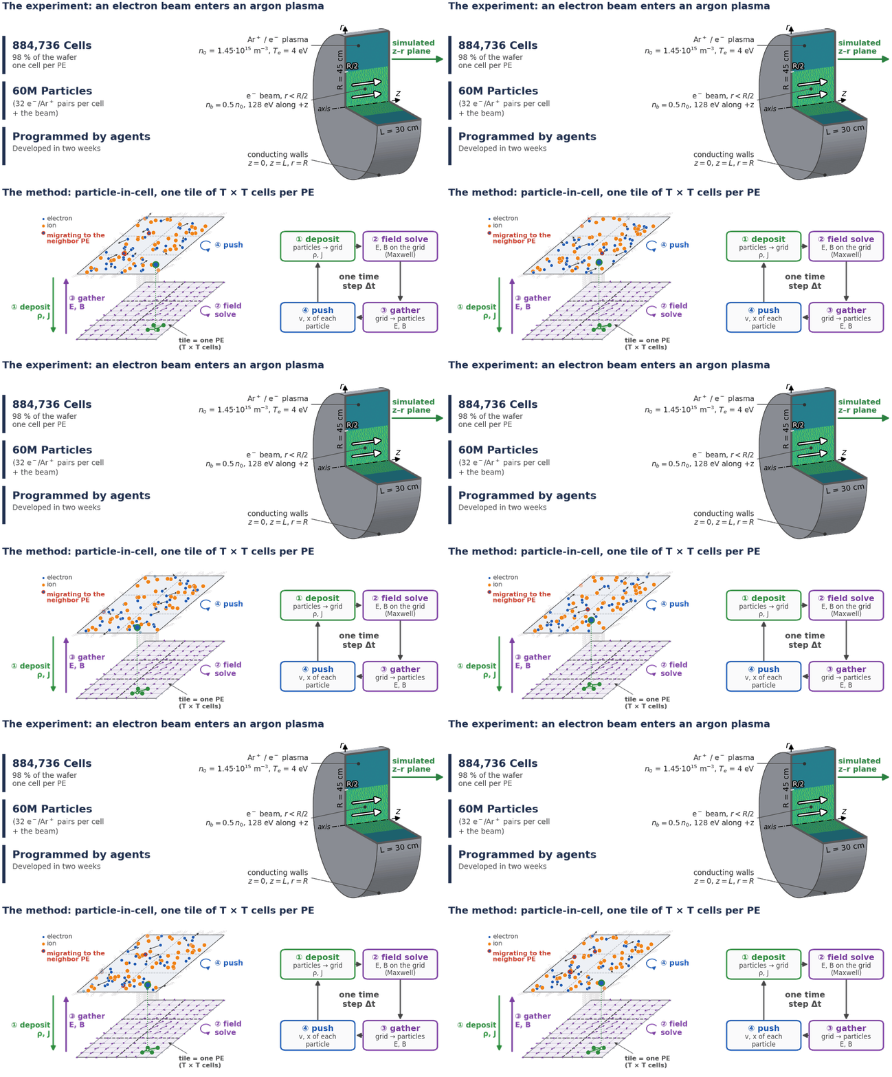
Figure 1. Top: the full-wafer experiment. An electron beam is fired into an argon plasma that fills a conducting cylinder; the simulation covers one z-r half-plane of the cylinder, with one cell per processing element (PE). Bottom: the particle-in-cell method. Particles (top layer) move freely, fields live on a fixed grid (bottom layer), and the two exchange information four times per time step. Each tile of the grid, and the particles above it, belongs to one PE.

Abstract

We present a two-dimensional, three-velocity (2D3V) electromagnetic particle-in-cell (PIC) code for the Cerebras Wafer-Scale Engine (WSE), a single silicon wafer carrying close to a million independent processors. Each processor owns one cell (or a small tile of cells) of the simulation mesh, the field values on it, and the particles inside it. All communication is between nearest neighbours. The code supports Cartesian (x-y) and axisymmetric (z-r) geometries. It offers an explicit Yee field solver and a θ-implicit Maxwell solver that allows time steps many times the light-wave stability limit. The implicit solver can use Chebyshev iteration, conjugate gradients, or conjugate gradients preconditioned with a geometric multigrid V-cycle. Particles are advanced with the Boris pusher, and their current is deposited with a charge-conserving zigzag scheme. Every run is checked against a single-threaded CPU reference written alongside it, and the two agree bit for bit: every field value and every particle coordinate, after every step.

We use the code for a full-wafer simulation on 884,736 PEs: an electron beam entering an argon plasma in a 30 cm × 45 cm metal cylinder, with 60 million macro-particles and 1500 implicit time steps. The run shows beam–plasma bunching, wall sheaths, a plasma return current that largely neutralizes the beam current, and long-lived electromagnetic cavity modes.

The code was written entirely by an AI coding agent, steered in conversation by a single researcher over about two weeks. Section 1 describes how, with the prompts that shaped it.

---

1. How this code was written

1.1 The working arrangement

No line of the code, test scripts, reference implementation, figures or documentation in this directory was typed by a human. The work was done by an AI coding agent (GitHub Copilot in agent mode, in VS Code). The agent read and edited files, ran the compiler and the simulator on a compute cluster, read their logs and memory dumps, and kept its own notes between sessions. A single researcher directed it through a chat window.

The division of labour settled quickly:

• The researcher chose the goals and the order of work, asked questions, made the judgment calls (which physics, which trade-offs, when a result was good enough), and ran the jobs on the wafer hardware, which the agent was not allowed to allocate.
• The agent proposed plans and answered the questions. It wrote the CPU reference and the wafer code, built the tests, found and fixed its own bugs, and turned each finding into tests and notes.

Most prompts are short. They steer rather than specify. The first prompt was sent on 26 September 2026, and the full-wafer run reported in Section 5 completed on 10 October 2026.

1.2 Prompts that shaped the application

The quotes below are examples of the researcher's prompts to the agent. They are verbatim, typos included, with dates. They are a small selection from a few hundred exchanges, chosen because each one changed the direction of the code.

Starting point. The project began with an existing open-source PIC code (XOOPIC) and a request to understand it.

"Please take a look at the files in this direcotory. It's a particle in cell code for plasma simulations that I'd like to understand and extract kernels from for porting to WSE platforms." (26 Sep)

A clean-room design. This decision set the method for everything that followed: textbook algorithms, an independent reference, and statistical comparison with the original code rather than a translation of it.

"Good advice, let's keep XOOPIC out of the project and let's not line-by line port the code but rather use texbook algorithms for creating a reference and Tungsten code. I asume we can still compare the results of the computation for statiscal match between our code an Xoopic without raising licencsing concerns." (26 Sep)

Two flows: explicit and implicit. The researcher set the tile size and split the work into an explicit flow for XOOPIC-class problems and an implicit one for EMPIRE-like problems.

"2x2 tiles are what we need, earlier analysis assumed that we use fewer per cell than we actually need. I think we should implement two separate flows: the current one for XOOPIC class problems and EMPIRE-like with implicit solver." (29 Sep)

Architecture from experience. The researcher contributed knowledge of the machine. This prompt fixed the design of the global reduction (Section 3.3).

"For CG, please use allreduce to/from the center of the used PE region. I have a standalone example if you need one." (30 Sep)

Seeing the physics. This prompt led to the on-device movie frames (Section 2.4).

"I'd like to explore extended physics and diagnostics (using small runs first); then we can do HW runs and corrsponding diagnostics. It will be good to save periodic state as frames that we can put into a movie." (1 Oct)

Choosing the geometry. The researcher asked the agent to lay out the options before prioritizing. The answer led to the axisymmetric z-r geometry, done electromagnetic first.

"The priority is z-r geometry. Between electromagnetic and electrostatic, we'll do both but to help me prioritize, please let me know which is closer to EMPIRE, which matches Xoopic, and which is easier to implement?" (1 Oct)

Onto the hardware. The researcher showed the agent the commands once, and it automated them as MODE=hw (Section 6).

"Let's configure the MODE=hw so I can run hw tests easily. The commands and env settings that I used were: [...] Please use this flow to automate HW runs in Makefiles" (2 Oct)

A small and a large test for each experiment.

"For each flavor of experiments, we should have small simulatable tests an full wafer tests" (12 Nov)

1.3 Observations on the process

• A bitwise reference made the agent productive. Exact agreement with an independent CPU code turns every test into a yes/no answer. When a test failed, the agent could compare before/after snapshots of each kernel and point at the first differing value. Without an exact reference, an agent (or a person) has to judge "close enough", and bugs hide behind noise.
• Small tests first, always. Most tests in test.rc run on 4 × 4 or 5 × 3 PEs in the simulator within a minute or two. The large decks reuse exactly the same code paths. The researcher repeatedly pushed for shorter tests when a run took too long.
• The human supplied context the agent could not see. That context was the state of the machine, the conventions of the team, and the intended use of the results. The agent supplied breadth and stamina: reading listings, tracing values across thousands of PEs, and rewriting a kernel many times.
• Notes outlive sessions. The agent kept short notes of facts it had verified, such as compiler quirks and hardware behaviour that the simulator does not show. It reread them at the start of each session, so long projects survived context limits and restarts.

---

2. The physical model

2.1 Equations

The code solves the Vlasov–Maxwell system with macro-particles:

• 2D3V: two spatial coordinates, three velocity components;
• species of arbitrary charge and mass (here electrons and singly charged argon ions, m_i/m_e = 72,820);
• equal macro-particle weights.

Fields are advanced on a uniform staggered (Yee) mesh. Each time step performs the four operations of Figure 1:

1. Deposit. Each particle's motion during the step is turned into a current on the mesh with the zigzag scheme of Umeda et al. This scheme is charge-conserving: Gauss's law remains satisfied to rounding error without any Poisson correction. The Villasenor–Buneman scheme is also available in the reference.
2. Field solve. Maxwell's equations are advanced by one step, explicitly (Yee) or implicitly (Section 2.2).
3. Gather. Fields are interpolated from the mesh nodes to each particle (bilinear, or cloud-in-cell).
4. Push. Velocities are rotated and accelerated with the Boris scheme (non-relativistic or relativistic), and positions are advanced.

2.2 Implicit fields

An explicit Yee scheme must resolve light: c Δt < Δx/√2. Low-temperature plasmas move far slower than light, so that limit wastes most steps. With the θ-implicit scheme (θ ∈ [½, 1]), each step reduces to two scalar 5-point Helmholtz problems, one for B_θ (or B_z) and one for E_θ (or E_z). The step size is then limited by the plasma frequency instead, and θ slightly above ½ damps the unresolved light modes.

Three solvers are implemented:

• Chebyshev iteration. The spectral bounds of the Helmholtz operator are known in closed form, so the iteration coefficients are precomputed and the solve needs no global reductions at all: every iteration is a stencil and a neighbour exchange. This is the solver of the full-wafer run.
• Conjugate gradients (CG). The iteration stops on a residual tolerance. Each iteration needs two global sums.
• CG preconditioned with a geometric multigrid V-cycle (PCG). It suits very stiff problems, such as time steps of 100 times the light limit.

2.3 Geometry and boundaries

• x-y. Doubly periodic, or with perfectly conducting walls on either pair of edges.
• z-r (axisymmetric). Here x is z and y is r. The axis is at r = 0, and the outer conducting wall at r = R. Every operator is r-weighted.
  • The particle move is exact: a straight line in the particle's local Cartesian frame, mapped back to (z, r), with (u_r, u_θ) rotated by the swept angle. Particles may cross the axis.
  • The currents are divided by r-weighted node volumes, with π Δr²/3 for the axis node.
• Walls. Tangential E is zero on a wall after every E update. A particle that crosses a wall is absorbed and counted.

2.4 Diagnostics and restart

• Movie frames. Every FEV steps, each PE adds its density per species, E_z (in z-r: E_r) and B_z (in z-r: B_θ) to a frame buffer in its own memory. The frames are read at the end of the run. They can be stored at full resolution or as one value per block of cells.
• Restart. A run can continue from the final device state of a previous run, so long movies can be stitched from chunks (picref/movie.py).

---

3. Mapping PIC onto a wafer

3.1 The machine

The WSE is a two-dimensional mesh of about 900,000 PEs. Each PE has:

• 48 KiB of private memory, which holds both its program and its data;
• a single-precision floating-point datapath;
• a router connected to its four neighbours.

There is no shared memory and no cache. A PE can compute while its router moves data, and a message to a neighbour costs a few clock cycles. The natural program is therefore one in which every PE owns a small piece of the problem and talks mostly to its neighbours.

Programs are written in Tungsten, the WSE kernel language (pic.w, k6i.w, arcore.w, moat.w). The placement of programs on PEs and the routes between them are described in .paint files (bench.paint, allred.paint).

3.2 Domain decomposition: one tile per PE

The W × H rectangle of PEs covers a mesh of (W·T) × (H·T) cells. Each PE owns a T × T tile; T = 1 (one cell per PE) is used at full scale. A PE holds:

• the six Yee field components and three current components of its tile, plus a one-cell halo on the low side and a two-cell halo on the high side;
• node-centred copies of the fields, interleaved so that the six values a particle needs at one node are adjacent in memory;
• for each species, a list of up to CAP particles: six single-precision rows, holding the position within the tile, three velocity components and an identifier;
• send buffers of MCAP particles per direction, for particles leaving the tile.

3.3 Communication: halos, migration and the moat

The code uses four bidirectional neighbour channels per PE (left, right, down, up). They carry three kinds of traffic:

• Halo fills. Field values are copied into the neighbours' halos before every stencil.
• Current reduction. After the deposit, each PE adds the current that its particles left in its halo cells to the owning neighbour's cells, in a fixed order.
• Particle migration. Particles that left the tile are compacted out of the list and sent across the edge in z (or x) first, then in r (or y), so diagonal moves take two hops. A particle may cross at most one tile per step, which the time step guarantees here. If a list or a send buffer is full, the particle is dropped and a flag is raised. The run still completes, and the check reports the flag.

Periodic boundaries. A periodic mesh needs links between opposite edges of the PE rectangle. These are provided by a moat: a ring of forwarding PEs around the grid (moat.w). A moat PE takes traffic leaving the edge of the grid and forwards it on a dedicated route across the whole grid to the moat on the opposite side, which injects it back as if it came from the periodic neighbour. With conducting walls the moat stays in place but carries no particles.

Global sums. These are needed only by CG and PCG, and by an optional barrier before the last step. They use an allreduce rooted at the centre of the grid (arcore.w, allred.paint):

1. Rows funnel their values towards a central column.
2. Columns funnel towards four quadrant roots.
3. The roots combine their sums in a fixed order and broadcast the total back over static routes.

The fixed summation order makes the result bitwise identical on every PE, and identical to the reference.

3.4 One program, one call site per kernel

Every PE runs the same program. Its role (interior, wall or axis tile, reduction role) is data that the host loads, not separate code. This keeps a single compilation for the whole grid.

The compiler inlines every function call, so a kernel called from two places costs twice the memory. The main loop of pic.w is therefore a small state machine over passes:

• particles and fields;
• the frame pass, which reuses the deposit and reduction machinery to accumulate densities;
• the first-step halo fill.

Each kernel appears exactly once.

3.5 Host side

The host does what is cheap on a CPU and awkward on a PE. host.py:

• builds the initial state;
• runs the reference;
• computes every floating-point constant: field scalings, z-r row tables, Chebyshev and multigrid coefficients (mghost.py);
• computes the reduction roles (arhost.py);
• writes the per-PE memory images.

Tables that are identical on every PE are written once and replicated (misetb.py).

---

4. Verification: bit-for-bit agreement with a CPU reference

4.1 The reference

picref/picref.c is a single-threaded C implementation of the same model, written from the published algorithms (Boris; Birdsall & Langdon; Villasenor & Buneman; Umeda et al.; Yee). In its tiled mode it imitates the decomposition of Section 3.2: it keeps per-tile particle lists in tile-local coordinates, migrates particles between tiles, and reduces currents in the device's order. It can also write before/after snapshots of every kernel for a chosen step, which makes the first differing value easy to find.

4.2 The arithmetic contract

Floating-point results depend on the order of operations. The two codes therefore follow one contract:

• No fused multiply-add. picref is compiled with -ffp-contract=off, and on the wafer every operation is written as its own statement, in picref's evaluation order.
• No division and no square root. Reciprocals and reciprocal square roots use the same bit-manipulation seed followed by a fixed number of Newton steps in both codes.
• Fixed summation order for the deposit within a tile, for the current reduction across tiles, and for every global sum.
• Host-computed constants. Every coefficient is computed once in single precision on the host and loaded into both codes.

4.3 What a test checks

Each line of test.rc is a test. A test:

1. builds the state;
2. runs picref;
3. loads the images;
4. runs the wafer program (on the simulator, or with MODE=hw on the machine);
5. reads back the memory of every PE.

The check then compares every field value, and every particle's position, velocity and identifier, for exact equality. A single differing bit fails the test. Frames and restart chains are compared too.

Runs too long for a CPU reference (CHK=0) get a sanity check instead:

• every PE finished every step;
• no overflow flag;
• every particle is inside its tile, with a finite value and a unique identifier;
• all fields are finite.

The 68 tests cover:

• both geometries, walls, and one, two or four cells per tile;
• both pushers;
• all four field solvers, and two species;
• capacity overflow;
• frames and restart chains;
• the experiment decks at three sizes.

4.4 Validation of the reference

picref was validated against the original XOOPIC program in three ways:

• kernel by kernel, against an independent single-precision implementation;
• over short horizons, starting from XOOPIC's own particle dumps;
• statistically, on ensembles of two-stream instability runs, where the observables agreed within sampling error.

The z-r geometry has its own physics tests: cavity eigenmodes against Bessel-function roots, density uniformity on every row including the axis, gyration orbits, Gauss's law and energy conservation.

---

5. Experiment: an electron beam in an argon plasma

5.1 Setup

The deck is a low-temperature argon plasma in a closed metal cylinder, modelled on a problem of the EMPIRE plasma code, with the cylinder enlarged to fill the wafer and an electron beam added along the axis.

Geometry	z-r cylinder, L = 30 cm (768 cells) by R = 45 cm (1152 cells); Δz = Δr = 391 µm = one Debye length. Conducting walls at z = 0, z = L and r = R
Plasma	n₀ = 1.45 × 10¹⁵ m⁻³ (ω_p = 2.15 × 10⁹ s⁻¹, c/ω_p = 14 cm). Electrons at 4 eV, argon ions at 0.03 eV. Each ion starts on top of an electron, so the charge density is zero at t = 0
Beam	Electrons at density 0.5 n₀ in r < R/2, over the full length. Drift along +z at 8 electron thermal speeds (128 eV, 0.022 c), with a 4 eV spread
Start	E = B = 0. The beam current switches on instantaneously
Particles	32 electron–ion pairs per cell on average: 31.9 M electrons (3.5 M of them in the beam) and 28.3 M ions, 60.2 M in total
Time step	ω_p Δt = 0.049, 25 times the explicit light-wave limit
Solver	θ = 0.55, Chebyshev, 233 iterations per step (relative error 10⁻⁶)
Run	1500 steps = 74/ω_p = 34 ns, with a frame every 15 steps
Machine	768 × 1152 = 884,736 PEs, one cell each: 98 % of the wafer

In units of the plasma skin depth, R = 3.2 c/ω_p and the beam radius is 1.6 c/ω_p. The beam is wider than the skin depth, so the plasma can carry a return current inside it.

Verification at full scale. The same deck run for 3 steps at 16 pairs per cell (test bwfc) matches picref bit for bit:

• all 884,736 values of each of the six field components;
• every coordinate of all 30 million particles;
• every frame value.

The halved particle count keeps the single-precision particle identifiers exact (below 2²⁴ per species). The 1500-step run (bwf) passes the sanity checks of Section 4.3.

5.2 Electron density

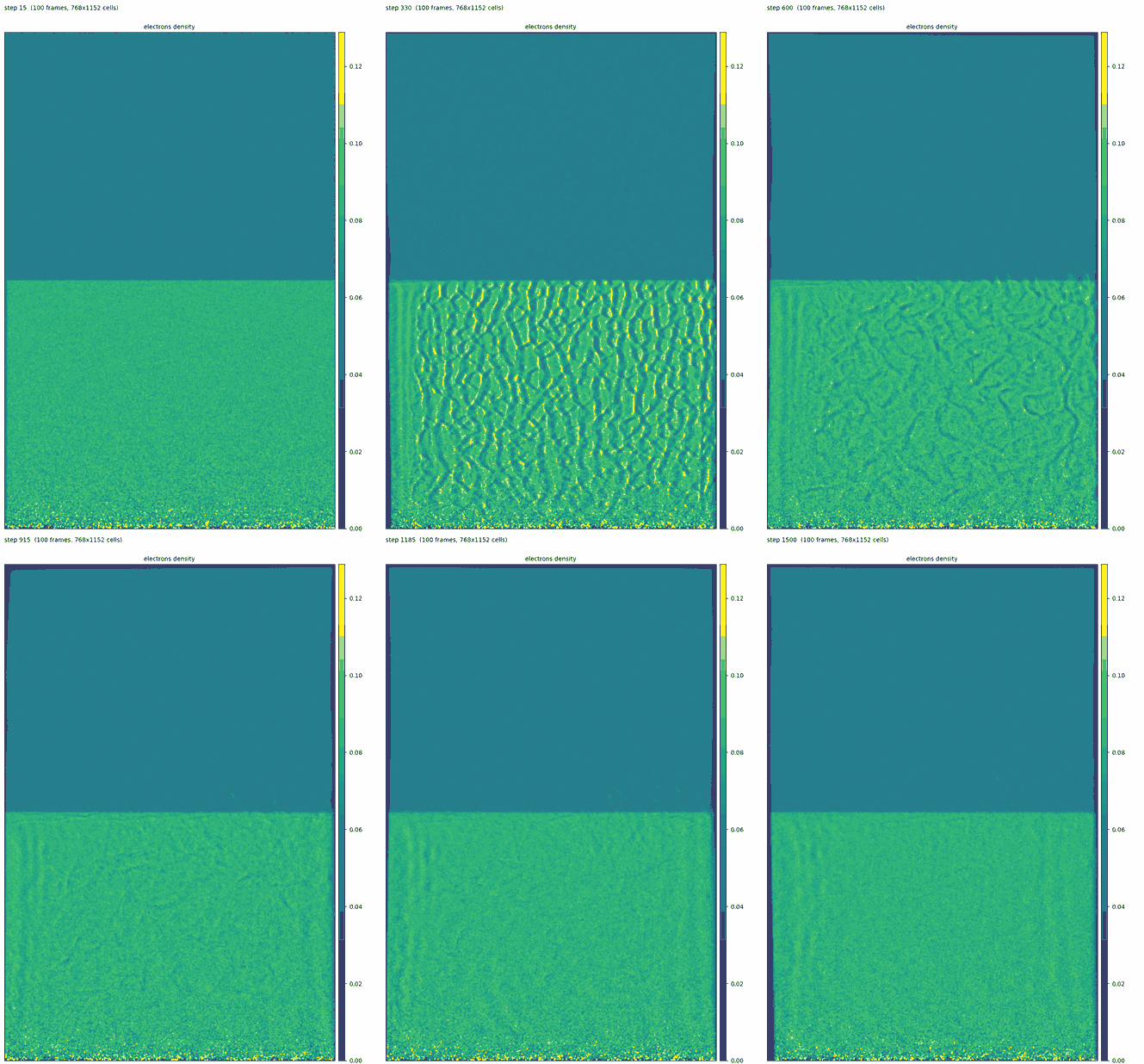
Figure 2. Electron density in the z-r half-plane, z to the right, r up, the axis at the bottom. The colour scale is fixed over the run. This animation shows every third stored frame, one per 45 steps, at half resolution.

• The beam column. The lower half of the picture (r < R/2) holds the beam on top of the background, at 1.5 n₀. Averaged along z, this contrast persists for the whole run. The beam is not blown apart radially, because its charge is neutralized by the plasma.
• Beam–plasma bunching. Axial density bunches grow in the beam column from the noise level to a 4–5 % modulation by t ω_p ≈ 5–15, at wavelengths of 23–31 Debye lengths. They then relax to about 1.5 % at longer wavelengths, 46–61 Debye lengths, close to the cold-beam resonance 2π v_b/ω_p ≈ 50 Debye lengths. Outside the beam the modulation stays at the 0.5 % noise floor.
• Sheaths. Electrons at 4 eV move only about 3 cm in the whole run, so wall effects stay in thin layers:
  • near r = R the electron density drops to 30–40 % of n₀, and a positive radial field of about 7.5 kV/m builds up;
  • near z = 0 a depleted layer forms, as the beam drifts away from that wall;
  • 3.4 % of the electrons and 0.07 % of the ions reach a wall during the run.
• Ions. The argon plasma period is about 1700/ω_p, far longer than the run, so the ion density stays uniform up to particle noise.

5.3 Magnetic field

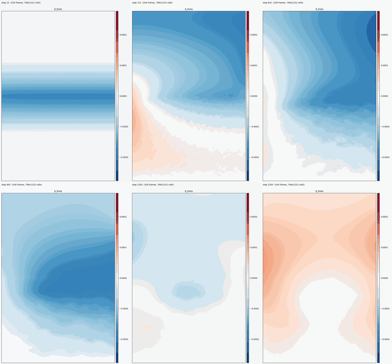
Figure 3. The azimuthal magnetic field B_θ, on a diverging colour scale (zero is the centre colour), every stored frame, at half resolution.

B_θ has two parts of similar size.

A steady part: the net current.

• B_θ is negative everywhere, as expected for electrons moving in +z.
• It is zero on the axis and peaks just inside the beam edge.
• Inside the beam it rises more slowly than the linear profile of an unneutralized beam.
• By Ampère's law, the late-time peak corresponds to a net axial current of about 26 A, against the beam's own 88 A. The plasma thus carries a return current that cancels about 70 % of the beam current, and it persists for the whole run.

An oscillating part: cavity modes. Most of the motion in Figure 3 is a weakly damped oscillation of about ±2 × 10⁻⁵ T at the beam edge, with E_r oscillating along with it. Frames taken every 5 steps resolve it into two spectral lines, near 1.4 ω_p and 2.0 ω_p. These match the lowest TM modes of a plasma-filled cylinder, ω² ≈ ω_p² + (2.405 c/R)² + (nπc/L)²: TM₀₁₀ ≈ 1.25 ω_p and TM₀₁₁ ≈ 1.9 ω_p. The modes are rung by the instantaneous switch-on of the beam current. The time step resolves them (ω Δt ≤ 0.1), so θ = 0.55 barely damps them.

5.4 Open questions

These are questions for plasma physicists rather than for the code:

• Would a ramped beam current, or injection from an emitter at z = 0, be a more meaningful setup than an instantaneous switch-on?
• How does the persistent 30 % net current compare with theory for a collisionless beam of this radius?
• What sets the early, shorter bunching wavelengths? The beam is strong (n_b/n₀ = 0.5) and of finite radius.

---

6. Running the code

6.1 Tests

From this directory, with the WSE SDK environment loaded:

make check GOAL=test TEST="s4 z4 bmzh"          # a few tests on the simulator (MODE=sim)
make -k -j16 check GOAL=test TEST="..."         # many tests in parallel

Each test runs in test-<name>/ and prints PASS <size>: bitwise vs picref (or the sanity check for CHK=0). The test parameters are the make variables documented at the top of the Makefile: grid, tile size, deck, solver, walls, geometry, frames and restart.

The medium decks (bmzc, bmzn, tsvc, tsvm) and the full-wafer decks (bwfc, bwf) are meant for the machine:

export CSCLIENT_DIR=/path/to/csclient        # holds csclient.py
export CSRTSERV=http://<run server>:<port>   # the run server
export HWBUNDLE=<allocated bundle>           # default: $USER-reg
make -k check GOAL=test TEST="bwfc bwf" MODE=hw

hwrun.py loads the image, waits for every PE to report completion, and fetches the result arrays. The bundle must already be allocated. Use make -k, so that one failing test does not stop the others. Restart chains (RESTART=../test-X) read the earlier test's directory, so do not make clean between the parts of a chain.

6.2 Movies

python3 picref/movie.py test-bwf --smooth 2 --split --fps 4 -o bwf.gif         # bwf_rho0.gif, bwf_rho1.gif, bwf_ey.gif, bwf_bz.gif
python3 picref/movie.py test-bwf --smooth 2 --tavg 5 --only ey,bz --split -o bwf_tavg5.gif   # running mean: the slow fields
python3 picref/movie.py test-a test-b -o chain.gif                            # stitch a restart chain

6.3 The reference on its own

picref can be used without the wafer:

gcc -O2 -std=c11 -ffp-contract=off -fno-fast-math -o picref/picref picref/picref.c -lm
python3 picref/mkstate.py empire --seed 1 --scale 4 -o state.prs     # 128 x 32-cell cylinder, 131 k particles
picref/picref -i state.prs -n 40 -T 2 -w x -F imp -t 0.55 -f 4 -o run_
python3 picref/movie.py run_frames.prs -o empire.gif

The header of picref/picref.c documents all options, the units, the staggering and the time levels.

6.4 Figures

python3 figures/pic_slide_fig.py bwf_rho0.gif -o pic_overview.png --anim pic_overview.gif   # Figure 1
python3 figures/experiment_fig.py bwf_rho0.gif -o bwf_diagram.png                           # the cylinder alone
python3 figures/pic_diagram.py pic_structure.png                                            # the method alone

The input is the full-resolution electron-density movie from Section 6.2.

---

7. Limitations

The following are not implemented:

• internal conductors and dielectrics;
• particle injection and emission;
• collisions (Monte Carlo collisions);
• external magnetic fields;
• variable macro-particle weights;
• per-species subcycling.

Particles may move at most one tile per step. Particle identifiers are single-precision and exact below 2²⁴ per species, which limits bitwise checks to about 16 M particles per species; long production runs use the sanity check instead.

---

8. Files

File	Content
pic.w	The PIC program of one PE: halos, node fields, push, move, deposit, migration, current reduction, Yee update, walls, z-r, frames, and the main-loop state machine
k6i.w	θ-implicit field solve: right-hand side, Chebyshev iteration, CG, PCG with the multigrid V-cycle, and the field update
arcore.w, allred.paint	Centre-rooted allreduce: per-PE code, routes and roles
moat.w	Moat PE: forwards traffic across the grid for periodic wrap
bench.paint	Layout: the PE grid, the moat ring, channel colours
Makefile, test.rc	Build, test parameters, and the test list
host.py	Builds the state, runs picref, writes PE images, checks results
mghost.py, arhost.py, misetb.py	Multigrid tables, allreduce roles, replicated-table loader
hwrun.py	Runs an image on the machine and fetches the results (MODE=hw)
picref/picref.c	The CPU reference
picref/mkstate.py	Initial states: two-stream, low-temperature plasma, the cylinder deck
picref/pr_io.py	State/dump file format, physical constants, unit conversion
picref/movie.py	Stitches frames from runs and renders movies
figures/	Figure scripts and the animations shown above

---

References

• J. P. Boris, "Relativistic plasma simulation — optimization of a hybrid code", Proc. Fourth Conf. Numerical Simulation of Plasmas (1970).
• C. K. Birdsall and A. B. Langdon, Plasma Physics via Computer Simulation, McGraw-Hill (1985).
• K. S. Yee, "Numerical solution of initial boundary value problems involving Maxwell's equations in isotropic media", IEEE Trans. Antennas Propag. 14, 302 (1966).
• J. Villasenor and O. Buneman, "Rigorous charge conservation for local electromagnetic field solvers", Comput. Phys. Commun. 69, 306 (1992).
• T. Umeda, Y. Omura, T. Tominaga and H. Matsumoto, "A new charge conservation method in electromagnetic particle-in-cell simulations", Comput. Phys. Commun. 156, 73 (2003).
• J. P. Verboncoeur, A. B. Langdon and N. T. Gladd, "An object-oriented electromagnetic PIC code" (XOOPIC), Comput. Phys. Commun. 87, 199 (1995).
• M. T. Bettencourt et al., "EMPIRE-PIC: a performance portable unstructured particle-in-cell code", Commun. Comput. Phys. 30, 1232 (2021).

Run it

The experimental SDK installs this project beside the tutorial, as projects/pic. Run it like a tutorial: tungsten-tutorials -f projects/pic.