Shallow-water equations

A wafer-scale solver for the linear shallow-water equations in two dimensions: gravity waves on a rotating plane in a closed square basin. Each processing element (PE) owns an $\mathrm{NC} \times \mathrm{NC}$ block of grid cells, exchanges the edges of its block with its four neighbours every time step, and advances every cell by one explicit step. A ring of moat tiles around the grid closes the basin. The scheme is second order in space and time and conserves mass to roundoff.

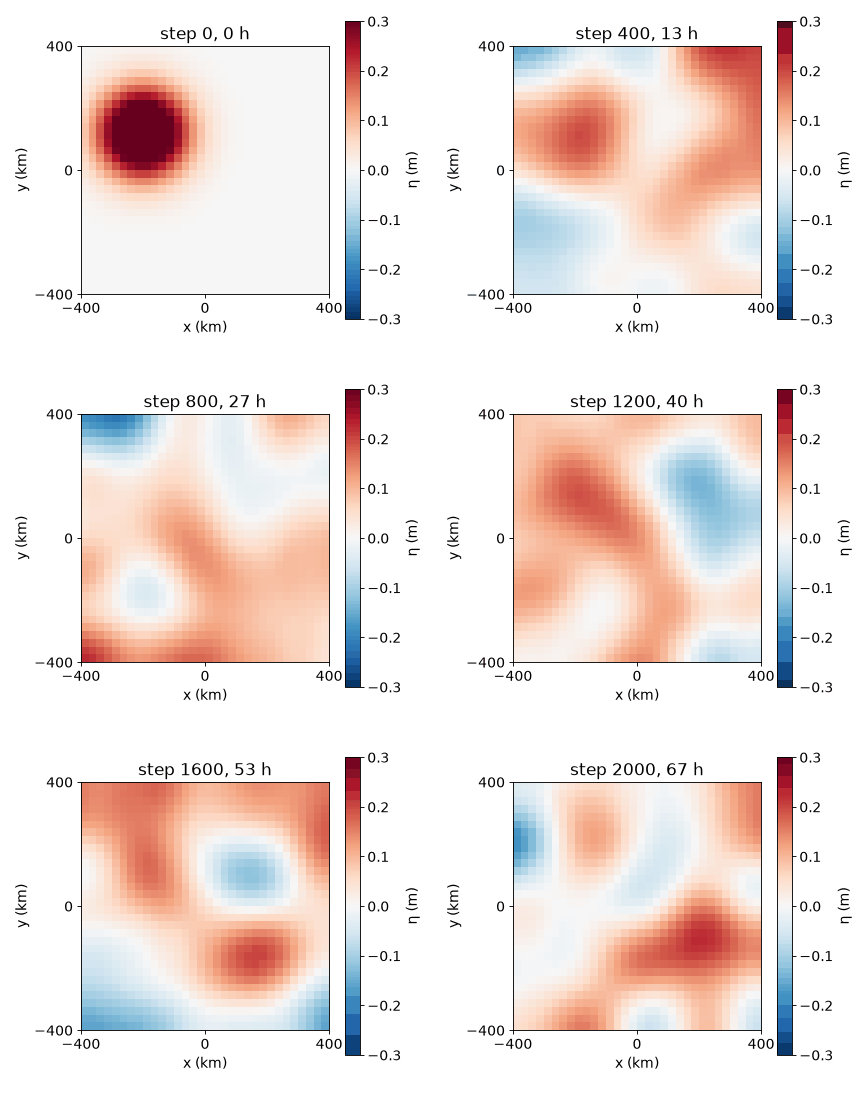
The surface height $\eta$ on the $32 \times 32$ grid every 50 steps (1.7 hours) over the first 2000 steps (67 hours). The colour scale stops at $\pm 0.3$ m, so the 0.5 m starting bump saturates in the first frame.

---

Algorithm

PDE

The unknowns are the surface elevation $\eta(x, y, t)$ above a resting depth $H$ and the depth-averaged velocities $u$, $v$. For waves much lower than the depth ($\eta \ll H$) the equations are linear:

$$\begin{aligned} \frac{\partial u}{\partial t} &= -g \frac{\partial \eta}{\partial x} + f v \\[2pt] \frac{\partial v}{\partial t} &= -g \frac{\partial \eta}{\partial y} - f u \\[2pt] \frac{\partial \eta}{\partial t} &= -H \left( \frac{\partial u}{\partial x} + \frac{\partial v}{\partial y} \right) \end{aligned}$$

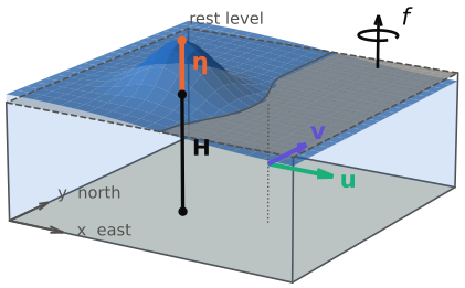
$H$ is measured from the flat bottom to the rest level (grey) and $\eta$ from the rest level to the free surface (blue), negative where the water is below the rest level; $u$ and $v$ are averaged over the water column. The Coriolis parameter varies with latitude, $f = f_0 + \beta y$ (a beta-plane). The bottom-friction terms $-ku$ and $-kv$ of the full linear equations are dropped, so the energy is conserved and the scheme can be checked against it.

Constant	Value		Constant	Value
$L_x = L_y$	800 km		$A$	0.5 m
$H$	100 m		$(x_0, y_0)$	$(-200, +120)$ km
$g$	$9.81\ \mathrm{m\,s^{-2}}$		$\sigma$	100 km
$f_0$	$10^{-4}\ \mathrm{s^{-1}}$		$\beta$	$2 \times 10^{-11}\ \mathrm{m^{-1}\,s^{-1}}$

The wave speed is $c = \sqrt{gH} = 31.3$ m/s and the Rossby radius $c/f_0 = 313$ km, about 40% of the basin, so rotation visibly bends the waves. Since $\eta/H \le 0.005$, the linear equations hold.

Discretisation

The basin is divided into $N_x \times N_y$ square cells of side $\Delta x = L_x/N_x$, with the variables staggered on an Arakawa C-grid: cell $(i, j)$ holds $\eta$ at its centre, $u$ on its east face and $v$ on its north face.

            v[i,j]
         +----^----+
         |         |
 u[i-1,j]>  eta    > u[i,j]
         |  [i,j]  |
         +----^----+
           v[i,j-1]

A difference of two neighbouring $\eta$ lands on the face between them, where the velocity it drives is stored, and the divergence of the four face velocities lands at the centre, where $\eta$ is stored. Both are centred, second order in $\Delta x$.

Rotation couples $u$ and $v$, which sit half a cell apart in each direction, so each equation uses the mean of the four values of the other velocity around its own point:

$$\bar v_{i,j} = \tfrac14 \left( v_{i,j} + v_{i+1,j} + v_{i,j-1} + v_{i+1,j-1} \right), \qquad \bar u_{i,j} = \tfrac14 \left( u_{i,j} + u_{i-1,j} + u_{i,j+1} + u_{i-1,j+1} \right)$$

  v̄ at the u point u[i,j]               ū at the v point v[i,j]

   v[i,j]          v[i+1,j]               u[i-1,j+1]      u[i,j+1]
     ^                 ^                      >               >
              x                                       x
     ^                 ^                      >               >
   v[i,j-1]        v[i+1,j-1]             u[i-1,j]        u[i,j]

Time integration

The scheme is forward-backward: the velocities are updated from the current $\eta$, then $\eta$ from the new velocities. On even steps $u$ goes first:

$$\begin{aligned} u^{n+1} &= u^n - \frac{g \Delta t}{\Delta x} \left( \eta^n_{i+1,j} - \eta^n_{i,j} \right) + \Delta t \, f \, \bar v^{\,n} \\[2pt] v^{n+1} &= v^n - \frac{g \Delta t}{\Delta y} \left( \eta^n_{i,j+1} - \eta^n_{i,j} \right) - \Delta t \, f \, \bar u^{\,n+1} \\[2pt] \eta^{n+1} &= \eta^n - H \Delta t \left( \frac{u^{n+1}_{i,j} - u^{n+1}_{i-1,j}}{\Delta x} + \frac{v^{n+1}_{i,j} - v^{n+1}_{i,j-1}}{\Delta y} \right) \end{aligned}$$

On odd steps $v$ goes first, from $\bar u^{\,n}$, and $u$ second, from $\bar v^{\,n+1}$. Three choices make the scheme second order in time:

1. Forward-backward for the waves. Using the new velocities in the continuity equation makes the $(u, \eta)$ pair behave like leapfrog, with the velocities half a step after $\eta$. It is stable for $c \Delta t \le \Delta x/\sqrt 2$; this model runs at $c \Delta t/\Delta x = 0.15$.
2. Alternating the order for rotation. Each order alone is first order; swapping it every step cancels the leading error over each pair of steps.
3. Starting the velocities half a step back. From rest, the host sets $u(-\Delta t/2) = +\tfrac12 g \Delta t \, \partial \eta/\partial x$ (at most 1.8 mm/s), and likewise $v$. Starting them at 0 leaves a $\Delta t/2$ offset that makes the run first order.

Each face velocity enters the two cells it separates with opposite signs, so $\sum \eta$ is conserved exactly. The energy $E = \tfrac12 \sum \left( H (u^2 + v^2) + g \eta^2 \right) \Delta x \Delta y$ oscillates by about 1% but does not drift.

Initial and boundary conditions

The initial state is a Gaussian bump with the half-step velocities above:

$$\eta(x, y, 0) = A \exp\!\left(-\frac{(x - x_0)^2 + (y - y_0)^2}{2\sigma^2}\right)$$

At $32 \times 32$, $\Delta x = 25$ km and $\Delta t = 119.7$ s, so the bump is $\sigma/\Delta x = 4$ cells wide. The host computes every constant in double and rounds it to float32: $g\Delta t/\Delta x = 0.0470$, $H\Delta t/\Delta x = 0.479$, and $\alpha = f \Delta t$ at the $u$ and $v$ points (0.01104 to 0.01293 from south to north). The kernel then only adds and multiplies.

The walls are cell faces: $u = 0$ on the west and east walls, $v = 0$ on the south and north walls. Two mechanisms enforce this:

• every moat tile (moat.w) replies 0 to every wavelet it receives, so a PE on the west or south wall reads a halo velocity of 0, the wall velocity;
• a PE on the east or north wall multiplies its own $u$ or $v$ by a 0/1 mask (mask_u, mask_v), so the face velocity it stores on the wall is 0.

Domain decomposition

$\mathrm{NX} \times \mathrm{NY}$ solver PEs each own an $\mathrm{NC} \times \mathrm{NC}$ block, so the grid is $(\mathrm{NX} \cdot \mathrm{NC}) \times (\mathrm{NY} \cdot \mathrm{NC})$ cells. Every array is $(\mathrm{NC} + 2) \times (\mathrm{NC} + 2)$: the own cells at local indices 1 to $\mathrm{NC}$, and a one-cell halo at 0 and $\mathrm{NC} + 1$ holding copies of the neighbouring PEs' edge cells. Local cell $(i, j)$ on the PE in fabric column $p_x$ and row $p_y$ is grid cell $(p_x \mathrm{NC} + i - 1,\ p_y \mathrm{NC} + j - 1)$.

Every cell runs the same operations in the same order whether its neighbour is in the block or in the halo, so $\mathrm{NC} = 1$, 2 and 4 give the same bits. The $32 \times 32$ grid takes $34 \times 34 = 1156$ tiles at $\mathrm{NC} = 1$ and $10 \times 10 = 100$ at $\mathrm{NC} = 4$.

Halo exchange

exchange_eta() sends each edge of eta to its neighbour and receives the four halos, all in one parallel block: in two serial blocks every PE would wait on its first send while its neighbour is still sending, and the grid would deadlock.

$\bar v$ and $\bar u$ reach one cell diagonally, so exchange_u() and exchange_v() also fill the halo corners, in two phases:

inline function exchange_u() {
    parallel {
        j in [1, NC+1) eastward[]  <- u[NC][j];
        j in [1, NC+1) westward[]  <- u[1][j];
        j in [1, NC+1) u[0][j]    <- eastward[];
        j in [1, NC+1) u[NC+1][j] <- westward[];
    }
    parallel {
        i in [0, NC+2) northward[] <- u[i][NC];
        i in [0, NC+2) southward[] <- u[i][1];
        i in [0, NC+2) u[i][0]    <- northward[];
        i in [0, NC+2) u[i][NC+1] <- southward[];
    }
}

The first phase fills the west and east halo columns. The second sends whole rows, $\mathrm{NC} + 2$ wavelets each, including those halo columns: a row sent north in phase 2 carries, at its ends, the values its PE received from the east and west in phase 1, so the diagonal neighbour's corner arrives in two hops, with no diagonal routes. There is no global barrier; each PE waits for its halo values, so no PE gets more than one exchange ahead of its neighbours.

Phases of one time step

The loop n in [0, NSTEP/2) runs two steps per pass, so NSTEP is even:

	step $2n$ ($u$ first)	step $2n+1$ ($v$ first)
1	exchange_eta()	exchange_eta()
2	momentum_u(), from the old $\bar v$	momentum_v(), from the old $\bar u$
3	exchange_u()	exchange_v()
4	momentum_v(), from the new $\bar u$	momentum_u(), from the new $\bar v$
5	exchange_v()	exchange_u()
6	continuity()	continuity()

Each update stores in place: momentum reads only the other velocity and $\eta$ from neighbours, and continuity reads only its own $\eta$.

Kernel (swe.w)

Arrays (memory) have ASCII names, eta, u, alpha_u, gdtdx; registers use the equations' symbols: ⁰ before the update, ¹ after, E W N S for neighbours and a bar for the four-point mean. For each cell of the block, momentum_u() loads its neighbours and applies the first line of the scheme:

v̄  <- 0.25:sp * ((v⁰ + vE) + (vS + vSE));
u¹ <- u⁰ - gΔt_Δx * (ηE - η⁰) + α * v̄;
u¹ <- u¹ * mU + 0.0:sp;
u[i][j] <- u¹;

mU is 0 on the east column and 1 elsewhere, so the wall face gets $u = 0$ with no branch; + 0.0 turns the -0.0 a negative value times 0 gives into +0.0. momentum_v() is the mirror image. continuity() then uses the new velocities:

η¹ <- η⁰ - (HΔt_Δx * (u¹ - uW) + HΔt_Δy * (v¹ - vS));
eta[i][j] <- η¹;

Cell $i$'s u¹ is cell $i + 1$'s uW, the same float32 value whether the two share a PE or not, so every interior face cancels in $\sum \eta$.

Layout (bench.paint)

The fabric rectangle is $(\mathrm{NX} + 2) \times (\mathrm{NY} + 2)$ tiles: the solver PEs, a one-tile moat ring and four idle corners. Fabric x runs along $i$ (east), y along $j$ (north).

 y  +---+---+---+---+---+---+
    |   | m | m | m | m |   |     m  moat tile, moat.w
    +---+---+---+---+---+---+     s  solver PE,  swe.w
    | m | s | s | s | s | m |
    +---+---+---+---+---+---+     NX = NY = 4
    | m | s | s | s | s | m |
    +---+---+---+---+---+---+
    | m | s | s | s | s | m |
    +---+---+---+---+---+---+
    | m | s | s | s | s | m |
    +---+---+---+---+---+---+
    |   | m | m | m | m |   |
    +---+---+---+---+---+---+  x

Colors. Each direction of travel gets a receive color and a send color, because every tile both sends east and receives from the west on the same socket, and one color cannot have two sources (the core and the west port) in one router:

let a  = color()    (* recv from west  *)
let ap = color()    (* send east       *)

b/bp (westward), c/cp (northward) and d/dp (southward) follow the same pattern.

Routing: exactly one hop. Every tile gets the same two rules per direction. For eastward travel:

fabric : paint(ap [CXR|R])
fabric : paint(a  [L|LXC])
fabric : colorpair(a ap)

X swaps to the partner color, so a wavelet sent on a leaves east as ap and the next tile delivers it to its core as a: exactly one hop, which is what the stencil needs. |R and L| cut the routes at the rectangle's edge. Both kernels bind the same sockets, so a moat tile's reply returns on the halo's channels:

Socket	Colors	Sends to	Receives from
eastward	a/ap	east (+x)	west
westward	b/bp	west (−x)	east
northward	c/cp	north (+y)	south
southward	d/dp	south (−y)	north

Moat and interior. The outer ring runs moat.w and the interior runs swe.w, with the same socket bindings:

let moat = union( rect(0      0      NX+2 1)
                  rect(0      NY+1   NX+2 1)
                  rect(0      1      1    NY)
                  rect(NX+1   1      1    NY) )
moat : code('moat [eastward:a westward:b northward:c southward:d])

let interior = rect(1 1 NX NY)
interior : code('swe [eastward:a westward:b northward:c southward:d NSTEP:NSTEP NC:NC])
interior : name('grid)

name('grid) gives every solver PE's arrays the grid.<symbol> paths that miset and miget use.

Moat tiles (moat.w)

Each moat tile answers every wavelet with 0:sp, on the socket paired with the one it arrived on. One forever dispatch per direction, all four in one parallel block:

forever dispatch(westward) {      // from the interior to the east: west moat
    wavelet() {
        eastward[] <- 0:sp;
    }
}

That single reply closes all four walls:

Wall	What the solver PE next to it does with the reply
west, south	receives $u = 0$ ($v = 0$) in its halo: the wall velocity, so no water crosses, and the value $\bar v$, $\bar u$ use there; the $\eta$ it receives is never read
east, north	sets its own $u$ ($v$) to 0 with mask_u (mask_v), so the reply only reaches values the mask replaces

Every solver PE sends and receives all four ways, so the code is the same on every PE, and every send to a moat tile is matched by its reply: none is left queued for the next exchange. The four corner tiles receive nothing, since only cardinal neighbours send.

---

Source files

File	Role
swe.w	solver PE, one $\mathrm{NC} \times \mathrm{NC}$ block: halo exchanges, momentum with averaged rotation, walls, continuity
moat.w	moat tile: replies 0 to every wavelet
bench.paint	layout: colors, routing, moat ring, solver grid
swe_model.py	constants, initial state, float32 Mirror, 64-bit reference(), energy()
make-input.py	writes the 11 init-<symbol>.bin files
check-output.py	tier 1, tier 2, mass and energy
convergence.py	observed order of accuracy against the exact standing wave
Makefile, test.rc	build, load, run, check; the test rows

Host model

swe_model.py: Mirror repeats swe.w operation for operation in float32; FUSED lists the sites the compiler fuses into one multiply-add (only the two wall masks); reference() is the same scheme in double, written independently on face arrays; tile() lays a field out in the miset order "y x i j _word", halo included.

---

Parameters

Set per row of test.rc. PAINTVARS = NX NY NSTEP NC passes them to paint.

Variable	Meaning
NX, NY	solver PEs in x and y
NC	cells per PE along x and along y (default 1); the grid is $(\mathrm{NX} \cdot \mathrm{NC}) \times (\mathrm{NY} \cdot \mathrm{NC})$ cells, at least 2 each way
NSTEP	time steps run by one kernel launch; even
ARCH	sdr (WSE-3)

CYCLES (default 3,000,000) caps the simulation and THREADS sets the simulator's threads.

---

Building and running

The experimental SDK installs this example at <sdk>/share/tutorial/projects/swe/, where <sdk> is the SDK's directory. Run every row with tungsten-tutorials -f projects/swe, or work by hand in a copy of the directory, with <sdk>/bin on PATH and FLUTEMK, TESTMK and SIMFABRIC set as for the tutorials:

cp -r <sdk>/share/tutorial/projects/swe . && cd swe

make TEST=smoke               # build, simulate and check one row
make TEST='*'                 # every active row
make TEST=6                   # the commented-out full run (line 6), 27 min on 16 cores
make TEST=smoke GOAL=fma      # which float32 operations were fused
python3 convergence.py        # order of accuracy against the exact standing wave
make clean                    # remove all test-*/ directories

Each row builds in test-<tag>/: make-log holds the transcript and the checker's report, sim-{eta,u,v}.bin the results, bench-sim.log the cycle count.

Correctness check

check-output.py reads back eta, u and v and checks:

Test	Against	Passes when
tier 1	Mirror, float32, operation for operation	every bit equal
tier 2	reference(), in double	$\lvert d \rvert \le 10^{-5} + 10^{-4} \lvert x \rvert$
mass	the initial $\sum \eta$	relative drift $\le 10^{-4}$
energy	the initial $E$	reported only

Row	Cells	PEs × NC	Steps	tier 1	tier 2, max error in $\eta$ (m)	mass drift
smoke	$4 \times 4$	$4 \times 4 \times 1$	2	exact	2.6e-08	2.2e-08
rect	$6 \times 4$	$6 \times 4 \times 1$	4	exact	1.4e-08	1.2e-08
rect-nc2	$6 \times 4$	$3 \times 2 \times 2$	4	exact	1.4e-08	1.2e-08
n8	$8 \times 8$	$8 \times 8 \times 1$	50	exact	4.8e-08	3.1e-08
n8-nc4	$8 \times 8$	$2 \times 2 \times 4$	50	exact	4.8e-08	3.1e-08
full	$32 \times 32$	$8 \times 8 \times 4$	5000	exact	9.0e-07	1.1e-07

rect is not square, so an x/y swap fails; the nc rows give the same bits as one cell per PE; in 50 steps on $8 \times 8$ the wave reaches all four walls. Over the full run's 5000 steps (6.9 days) the energy ends at $E/E_0 = 0.998$. The same run with $\mathrm{NC} = 1$ on $32 \times 32$ PEs gives the same bits in 766 cycles per step, against 2,287 at $\mathrm{NC} = 4$: blocks trade cycles for tiles.

References

• Sockets
• Parallel blocks
• Functions
• Dispatch blocks
• Paint color pairs
• Paint color swap modifiers

Run it

The experimental SDK installs this project beside the tutorial, as projects/swe. Run it like a tutorial: tungsten-tutorials -f projects/swe.