SNAP: particle transport sweeps

SNAP is a proxy application from Los Alamos National Laboratory for deterministic particle transport. Its core is the sweep: every cell of a spatial grid receives particle fluxes from its upwind neighbors, computes how many particles scatter or are absorbed inside it, and sends the outgoing fluxes to its downwind neighbors. On conventional clusters, sweep codes are dominated by machinery for blocking, message packing and tuning. This project runs SNAP's 2D steady-state sweep with one spatial cell per PE, written the way the algorithm is usually described: receive, compute, send.

On a WSE-3, at the largest problem that fits (1,100 directions and 21 groups per cell on 766 × 1,170 PEs), this sweep sustains 962 TFLOP/s, 71.6% of FP32 peak. A variant that spreads each cell over a 2 × 2 tile of PEs sustains 1,003 TFLOP/s, 74.6% of peak. Both were built with a development version of the compiler with experimental optimization passes, which schedules a grind in 29 cycles. With the compiler in this toolset, a grind takes about 34 cycles.

The problem

SNAP tracks angular fluxes, the average number of particles crossing each cell in each of a fixed set of directions, the discrete ordinates. In 2D the directions fall into four quadrants, northeast, northwest, southwest and southeast, with $D$ directions in each. Particles are also divided into $G$ energy groups.

A sweep visits every direction of every quadrant and every group. For one direction, a cell with incoming fluxes $\psi_x$ (from its west or east neighbor) and $\psi_y$ (from its south or north neighbor) has the cell flux

$$\psi_c = \frac{S + \alpha_x \psi_x + \alpha_y \psi_y}{\sigma_t + \alpha_x + \alpha_y}, \qquad \psi_x^{\text{out}} = 2\psi_c - \psi_x, \qquad \psi_y^{\text{out}} = 2\psi_c - \psi_y,$$

where $\alpha_x = 2|\mu|/\Delta x$ and $\alpha_y = 2|\eta|/\Delta y$ come from the direction's cosines and the cell size, $\sigma_t$ is the cell material's total cross section, and $S$ is the source in that direction. The outgoing fluxes become the downwind cells' incoming fluxes, so each direction and group crosses the grid as a diagonal wavefront.

Scattering couples the directions. SNAP represents the source and the solution by $M$ moments, the coefficients of an expansion in functions of the direction like spherical harmonics, with $M = L(L + 1)/2$ for scattering order $L$. The source in one direction is a dot product of the source moments with that direction's expansion coefficients, and each cell flux adds its contribution back into the flux moments:

$$S = \sum_m q_m\, e_m, \qquad \phi_m \mathrel{+}= w\, \psi_c\, e_m .$$

The work for one cell, one direction and one group is a grind. With the default scattering order $L = 4$, so $M = 10$, a grind is 47 floating-point operations: two values received, two sent, and two dot-product-sized updates of local memory.

The program stores its inputs pre-scaled so that a grind needs no division. For each direction it keeps $\beta = \alpha_y/\alpha_x$, and for each direction, group and cell $a = 2\alpha_x / (\sigma_t + \alpha_x + \alpha_y)$. The fluxes on the fabric are scaled by $\sqrt{w\alpha_x}$ and the expansion coefficients by $\sqrt{w/\alpha_x}$. With these scalings the cell update becomes

$$\psi_c = (q + \psi_x + \beta\psi_y)\,a, \qquad \psi_x^{\text{out}} = \psi_c - \psi_x, \qquad \psi_y^{\text{out}} = \psi_c - \psi_y,$$

and the moment update needs no weight. generate_inputs.py computes these scaled inputs.

A solve runs NUM_OUTER_ITERS outer iterations, which recompute scattering between groups, each with NUM_INNER_ITERS inner iterations, which recompute scattering within each group and then sweep all four quadrants once.

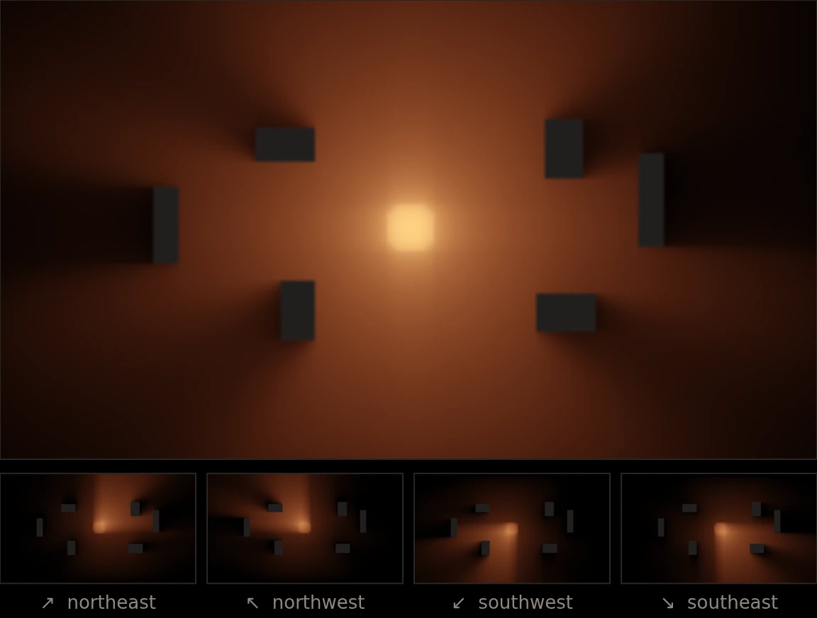
The same sweep on a small problem: a source in a medium where nine in ten collisions scatter, with six absorbing blocks, on 192 × 108 cells with 16 directions per quadrant. Each small panel shows the flux travelling in one quadrant's directions, and the large panel shows their sum. The first inner iteration carries only the particles that come straight from the source, which leaves sharp shadows behind the blocks. Each later iteration also includes particles that have scattered one more time, so the shadows fill in. The quadrant order alternates between iterations, as described below. For brevity the problem has one group, isotropic scattering and step differencing, $\psi_x^{\text{out}} = \psi_y^{\text{out}} = \psi_c$.

One cell per PE

The grid of cells maps directly onto the grid of PEs: PE $(x, y)$ holds cell $(x, y)$, with its material data, its source moments q_inner[g][m] and its flux moments flux_moments[g][m]. Every PE also holds the expansion coefficients ec[d][m] and the ratios beta[d].

Fluxes travel on two colors, one for each axis. Every PE sends its outgoing $x$ and $y$ fluxes on tx_x and tx_y, and receives its incoming fluxes on rx_x and rx_y. Which neighbor each of these sockets connects to depends on the quadrant: toward the northeast, rx_x receives from the west and tx_x sends to the east, and toward the northwest the other way around. The PE program never names a direction; the routers switch the routes at each change of quadrant, as the next section describes.

A flux value is one wavelet. Every PE iterates over quadrants, directions and groups in the same order, and the fabric delivers wavelets in the order they were sent, so the position of a value in the stream identifies it. There are no tags, no message buffers and no block sizes.

The grid's boundary is a vacuum: no particles enter from outside. The fabric handles the boundary, so that every PE of the grid runs exactly the same code, snap.w, whether it lies in the middle of the grid or on its edge. A ring of ghost PEs surrounds the grid, and each runs ghost.w. In the quadrants in which particles enter the grid from its side, a ghost sends one zero for every flux a neighbor would have sent:

∀k in [0, 4) {
    xp quadrant = k ^ mask;
    if (quadrant == FIRST || quadrant == SECOND) {
        ∀n in [0, NUM_DIRECTIONS * NUM_GROUPS) tx[] <- zero;
        tx[] <- control(ADV);
    }
}

Fluxes that leave the grid go nowhere: the routes on the grid's edges drop them, as the next section shows. The ghost ring costs two rows and two columns of PEs.

Switching the routes

A router can switch a color between up to four routes, called positions. In bench.paint, the $x$ color has one position per quadrant:

let [tx_x rx_x] = color()
grid : paint(tx_x [CHR|R ; CHL|L ; CHL|L ; CHR|R ; ring])
grid : colorpair(rx_x tx_x)

In the quadrant order northeast, northwest, southwest and southeast, $x$ fluxes travel east, west, west and east, and $y$ fluxes north, north, south and south. ring makes each switch return to its first position after its last. CHR|R sends to the right except from the grid's rightmost column, so a flux that would leave the grid is dropped. The receiving routes switch the same way:

grid : paint(rx_x [LHC ; RHC ; RHC ; LHC ; ring])

On the grid's west column, LHC receives from the ghost PE in the eastward quadrants.

A switch advances to its next position when a control wavelet passes through it. After its last flux of each quadrant, every PE sends one on each of its two colors:

tx_x[] <- control(ADV);
tx_y[] <- control(ADV);

The control wavelet travels behind the PE's last flux of the quadrant on the same color, so it cannot overtake it. It advances two switches: the sender's own route for tx_x and the downwind neighbor's route for rx_x. Each switch therefore moves exactly when the last flux of the quadrant has passed it, and the next quadrant's fluxes take the new route. A ghost PE sends the same control wavelet after its zeros, for the grid PE next to it. A change of quadrant costs a few cycles.

The grind loop

Here is the sweep in its simplest form. Every PE runs it, in every quadrant, because the routes, not the program, decide where fluxes come from and go:

∀d {
    ∀m ec_row[m] <- ec_walk[] * ec_sign[m];
    sp beta_d = beta[d];
    ∀g {
        sp q_acc <- expand();
        sp psi_x <- rx_x[];
        sp psi_y <- rx_y[];
        sp psi_c <- (q_acc + (psi_x + beta_d * psi_y)) * ax[d][g];
        tx_x[] <- psi_c - psi_x;
        tx_y[] <- psi_c - psi_y;
        contract(psi_c);
    }
}

Each iteration of the g loop is one grind. expand() computes the directional source, a dot product of the cell's source moments with the direction's expansion coefficients, and contract(psi_c) adds the cell flux back into the flux moments. Both are defined in snap.w:

iterator fm_walk = ∀inf ∀g ∀m flux_moments[g][m];
iterator qi_walk = ∀inf ∀g ∀m q_inner[g][m];

function expand() -> sp { sp result <- ∑m qi_walk[] * ec_row[m]; return result; }
function contract(sp psi_c) { ∀m fm_walk[] <+- psi_c * ec_row[m]; }

fm_walk and qi_walk walk the moment arrays group by group, so a sweep over all groups reads each array once in order, and they start again at the next direction. The first line of the direction loop copies the direction's expansion coefficients into ec_row, with the signs that the quadrant gives them.

Reading rx_x[] waits until the value from the upwind neighbor arrives. The hardware does the waiting: there is no polling, no lock and no barrier, so the arrival of data is the only synchronization the sweep needs.

Software pipelining

In the loop above, the values a PE sends depend on the values it receives, and its downwind neighbors wait for them. The cell flux also depends on the directional source that expand() computes in the same iteration, an $M$-term dot product. So every grind runs one chain of dependent operations, from the dot product through the cell flux to the sends, and each step waits for the result of the one before it. Yet the directional source does not depend on the received fluxes at all.

Software pipelining moves that work across iterations. The cell flux splits into a part known before the inputs arrive and a part that needs them,

$$\psi_c = q\,a + a\,(\psi_x + \beta\psi_y),$$

and the loop computes the next group's source while it waits for the current group's inputs. This is the direction loop in snap.w:

∀d {
    ∀m ec_row[m] <- ec_walk[] * ec_sign[m];
    sp beta_d = beta[d];
    q_acc <- expand();
    ∀g1 {
        sp ax_dg <- ax[d][g1];
        sp psi_c <- q_acc * ax_dg;
        q_acc <- expand();
        contract(upwind(psi_c, ax_dg, beta_d));
    }
    sp ax_dg <- ax[d][NUM_GROUPS - 1];
    contract(upwind(q_acc * ax_dg, ax_dg, beta_d));
}

The first expand() before the loop is the prologue; the g1 loop runs over the first $G - 1$ groups, each computing q_acc for the group after it; and the code after the loop is the epilogue for the last group, whose source is already computed. The inline function upwind() finishes the grind: it receives the upwind fluxes, completes the cell flux and sends the downwind fluxes.

inline function upwind(sp psi_c, sp ax_dg, sp beta_d) -> sp {
    sp psi_x <- rx_x[];
    sp psi_y <- rx_y[];
    psi_c <+- ax_dg * (psi_x + beta_d * psi_y);
    tx_x[] <- psi_c - psi_x;
    tx_y[] <- psi_c - psi_y;
    return psi_c;
}

Between a grind's receives and its sends there are now only the operations that need the received values: one fused multiply-add for $\psi_x + \beta\psi_y$, one for the cell flux, and two subtractions.

With the compiler in this toolset, the pipelined loop takes about 34 cycles per grind and the simple loop about 37. The 29-cycle grind of the full-wafer runs pipelines several grinds at once and needs the experimental compiler passes as well.

This transformation is written by hand for now. We intend the compiler to perform it automatically, so that the simple loop of the previous section compiles to the pipelined schedule.

Quadrants and sweep order

The four quadrants share one table of expansion coefficients, ec[d][m]. A coefficient's sign depends on the signs of the direction's cosines, and the same sign pattern applies to every direction of a quadrant. Before the solve, init_signs() builds one row of signs per quadrant in signs[4][m], and at the start of each quadrant the PE copies that quadrant's row into ec_sign:

∀k in [0, 4) {
    xp quadrant = k ^ mask;
    ∀m ec_sign[m] <- signs[quadrant][m];
    ∀d {
        ...
    }
    tx_x[] <- control(ADV);
    tx_y[] <- control(ADV);
}

The quadrant loop has no branches: all four quadrants run the same direction loop.

Each change of quadrant drains the wavefront from one corner of the grid and fills it from another, which leaves some PEs idle. The program reverses the quadrant order on every other inner iteration, northeast, northwest, southwest, southeast and then southeast, southwest, northwest, northeast, so consecutive sweeps meet in the same quadrant and one drain and fill disappears:

mask = 3 - mask;
∀k in [0, 4) {
    xp quadrant = k ^ mask;
    ...
}
tx_y[] <- control(ADV);
tx_y[] <- control(ADV);

The routes follow the reversal without a second set of positions. In the reversed order $x$ fluxes again travel east, west, west and east, so four advances per sweep bring the $x$ switch back to where the next sweep starts. $y$ fluxes travel south, south, north and north, so after each sweep the $y$ switch advances two positions further. The ghost PEs on the south and north sides send the same two extra control wavelets for the grid's first and last rows.

Source files

File	Contents
snap.w	The program every PE of the grid runs: its arrays and iteration ranges, the moment walks, expand and contract, the quadrant sign rows, the outer and inner source computations, upwind(), and the quadrant loop with the software-pipelined grind loop
ghost.w	The program of the ghost PEs around the grid, which send zero fluxes into it
bench.paint	The grid and its ghost ring, the two switching colors, and the regions that the input and output arrays are named by
generate_inputs.py	Builds the problem and writes each region's scaled input arrays
snap_ref.py	The reference implementation of SNAP's 2D steady-state solve that generate_inputs.py and validate.py use
validate.py	Reads the flux moments out of the simulated image and compares them with the reference
Makefile	Problem parameters, input generation, image patching and the test
test.rc	The test configurations

Each PE also records the cycle counter at the start and at the end of the solve in timestamps.

Parameters

Variable	Meaning	Default
NX, NY	Grid size in cells, which is also the size of the PE grid	16, 16
NUM_DIRECTIONS	Directions per quadrant, $D$	8
NUM_GROUPS	Energy groups, $G$	4
SCATTERING_ORDER	Scattering order $L$, at least 2; the program uses $L(L+1)/2$ moments	4
NUM_OUTER_ITERS	Outer iterations	3
NUM_INNER_ITERS	Inner iterations per outer iteration, one sweep each	6
SRC_OPT	SNAP's fixed source: 1, a unit source in the central quarter of the grid; 2, in its southwest quarter	1
MAT_OPT	SNAP's materials: 0, one material; 1, a second material in the central quarter; 2, in the southwest quarter	0

Building and running

make check TEST=<row> builds one configuration of test.rc, simulates it and validates the result; make check TEST='*' runs them all.

Row	Configuration
s1m2	16 × 16 cells, 8 directions, 4 groups
g16	8 × 8 cells, 4 directions, 16 groups
d24	8 × 8 cells, 24 directions, 4 groups
rect	12 × 6 cells, a grid that is not square
g5	8 × 8 cells, 5 groups

Every row puts the source in the central quarter and a second material in the southwest quarter (SRC_OPT=1, MAT_OPT=2).

Correctness check

validate.py reads flux_moments from every PE of the simulated image and compares them with snap_ref.py, which runs the same fixed numbers of outer and inner iterations in double precision. It prints how many of the flux moments agree within relative errors of $10^{-7}$ to $10^{-3}$, and passes when at least 99% agree within $10^{-3}$.

Checked against SNAP's reference code in all of its preset 2D source and material configurations, the FP32 scalar flux agrees with the double precision reference within a relative error of $3.2 \times 10^{-6}$, and every higher moment within $1.6 \times 10^{-6}$ times its largest magnitude.

References

• R. J. Zerr and R. S. Baker, "SNAP: SN (discrete ordinates) application proxy," Los Alamos National Laboratory, LA-CC-13-016. https://github.com/lanl/SNAP
• K. R. Koch, R. S. Baker and R. E. Alcouffe, "Solution of the first-order form of the 3-D discrete ordinates equation on a massively parallel processor," Trans. Amer. Nucl. Soc., vol. 65, pp. 198–199, 1992.

Run it

The experimental SDK installs this project beside the tutorial, as projects/snap. Run it like a tutorial: tungsten-tutorials -f projects/snap.